Deploying DNNs to Edge Devices with NNabla for Mixed-Precision Inference

Compression methods in NNabla

For several years, we have been working on implementing neural network compression methods to NNabla. Our goal is to reduce the memory and/or computational footprint of deep neural networks (DNN)s in order to run them on less-powerful edge
devices like wearables or IoT.

NNabla already natively includes a wide range of methods for network compression. We use them to deploy networks for Sony products. Quantization functions and special layers, which can replace more computation-intensive affine/convolutional layers, reduce the network
footprint by a factor of 10 or more.

Today, the list of compression methods offered by NNabla is quite impressive. More specifically, the following compression methods are available:

a) Compact layers for DNN reduction

• Low-rank approximation of weight matrix:
  svd_affine,
  svd_convolution

• Low-rank tensor approximation:
  cpd3_convolution

• Pruning:
  prune

b) Quantization methods for DNN reduction

• Binary:
  binary_tanh,
  binary_sigmoid

• Fixed-point:
  fixed_point_quantize

• Min-max:
  min_max_quantize

• Power-of-two:
  pow2_quantize

• BinaryConnect [1]

• Binary Weight Networks [2]

• Incremental Network Quantization [3]

• and for each of them, dedicated affine and convolution layers exist (e.g., fixed_point_quantized_affine).

Quantization functions reduce the number of bits that we spend for each weight and can also yield a reduction in the latency or power consumption. Compact architectures on the other hand reduce the number of weights and the number of operations required to operate the DNN. Both approaches can be combined and yield networks that can be deployed to very small edge devices.

Mixed precision DNNs

In our recent paper “Mixed Precision DNNs: All you need is a good parametrization”, which has been accepted to ICLR 2020, we present our latest algorithm to extend the NNabla compression toolbox.

In order to use DNNs on device, practitioners typically have to manually choose a global bit width to which all the weights are quantized. The bitwidth is chosen to meet the hardware and application constraints: memory, latency, computations, accuracy. In the paper, we show, however, that better performances can be achieved if we optimize the number of bits used by each layer while respecting the given hardware and application constraints.

With the proposed method, it is possible to automatically learn an optimal bit width to use at each layer. This can be learnt by gradient descent at the same time as the network weights are learned. This implies that the mixed precision training is performed roughly within the same training time as usual training. The key to achieve this is to choose a good parametrization of the quantization.

Quantization

Let us first review neural network quantization. For example, fixed-point quantization of a number \(x\) is computed by

\( q = Q\left\lbrack x;\mathbf{\theta} \right\rbrack = \text{sign}\left( x \right)\left\{ \begin{matrix}
d\left\lfloor \frac{\left| x \right|}{d} + \frac{1}{2} \right\rfloor & \left| x \right| \leq q_{\max} \\
q_{\max} & \left| x \right| > q_{\max} \\
\end{matrix} \right.\ ,
\)

where
\(\mathbf{\theta} = \left\lbrack d,\ q_{\max},\ b \right\rbrack^{T}\) is a parameter vector containing the step size \(d\), maximum value \(q_{\max}\) and number of bits \(b\) used to encode the quantized values \(q\). Hence,
in order to use such quantization, we need to choose good values for \(\mathbf{\theta}\). Although rules-of-thumb exist to choose these values from weights that were trained without quantization, it is in general not straightforward and can be cumbersome — especially if we want to use different \(\mathbf{\theta}\)s for different layers as is the case for mixed-precision networks.

Mixed-precision networks refers to a network where different number of bits are used for each layer. Heuristically, practitioners know that the first layer requires more bits than the other layers and being able to learn this distribution would allow us to reduce the manual tweaking
required.

Mixed precision DNNs using differentiable quantization

Our ICLR 2020 paper “Mixed precision DNNs: All you need is a good parametrization” comes at the rescue. In this paper, we show that the elements in \(\mathbf{\theta}\) can be learned with gradient descent. Furthermore, as the elements in \(\mathbf{\theta}\) are dependent, we can choose different parametrizations and in the paper we show that there is one that makes it easy to learn optimal values.

Using our differentiable quantization scheme, we can train mixed-precision ResNet-18 and MobileNetV2 models on ImageNet, which have an average size of 4bit.

The following table shows our results:

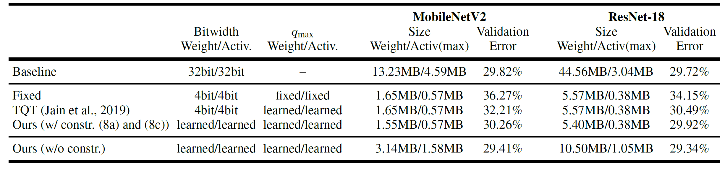
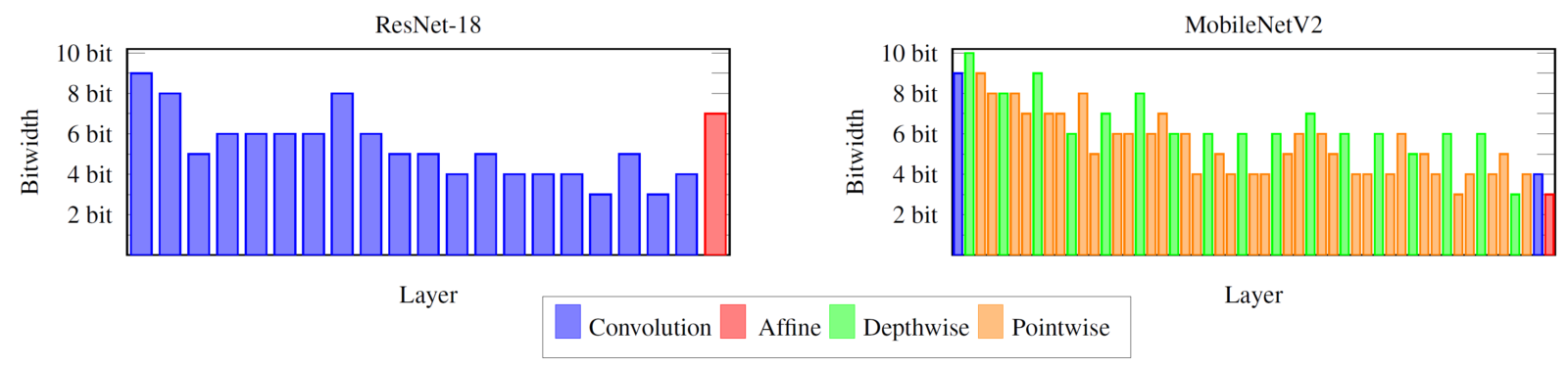
Our results compare favorably to other recent quantization approaches and it is interesting to see the learned weight bitwidth assignment:

Please check our paper or come to our poster at ICLR 2020 for more details and a comparison to other state-of-the-art quantization methods.

References

[1.] Courbariaux, Matthieu, Yoshua Bengio, and Jean-Pierre David.
“BinaryConnect: Training deep neural networks with binary weights
during propagations.” Advances in neural information processing
systems. 2015.

[2.] Rastegari, Mohammad, et al. “XNOR-net: ImageNet classification
using binary convolutional neural networks.” European Conference on
Computer Vision. Springer, Cham, 2016.

[3.] Zhou, Aojun, et al. “Incremental network quantization: Towards
lossless CNNs with low-precision weights.” arXiv preprint
arXiv:1702.03044 (2017).